Finding TTE and Sustained Efforts in a ride

Defining the problem

Any given training ride or race will contain periods of sustained effort, sometimes to exhaustion. Perhaps during the last sprint, or over a long climb, bridging a gap or chasing on after a roundabout or corner.

Being able to identify these efforts is rather useful.

The trouble is, deciding what represents a maximal or sustained effort is often discussed, and generally has fallen into discussions about intensity and FTP or Critical Power. These discussions have tended to then focus on trying to account for the interval duration, periods of freewheeling and applying smoothing etc.

But we already have an excellent description of what constitutes a maximal effort. It is the primary purpose of any power duration model.

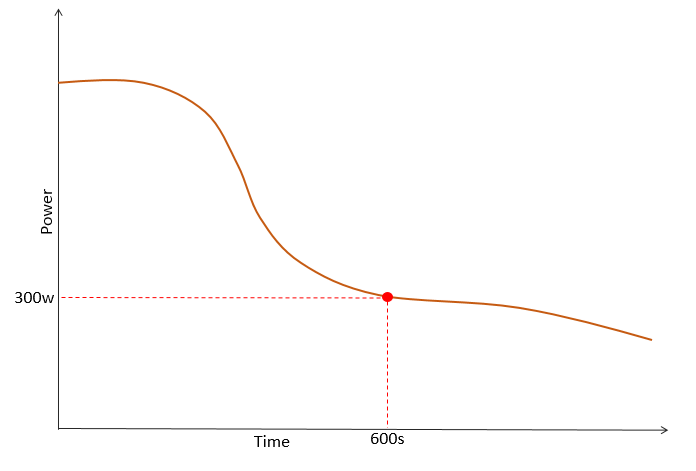
Power duration models estimate the maximal effort you can sustain for any given duration through to exhaustion. So if you want to identify maximal efforts its your friend.

Using the model below we can see, for example, that the athlete it represents could sustain 300 watts for 10 minutes before having to stop with exhaustion. So a time-to-exhaustion (TTE) of 10 minutes at 300 watts.

A sustained interval, is going to be similar; it will lie on or near the points on this curve.

And so, the problem of finding maximal efforts is quite easy to define (we will come back to sustained intervals at the end):

Identify intervals of any duration whose average power is equal to (or higher) than the estimate from your chosen power duration model.

Solving the problem

The problem is not difficult to solve. You could simply iterate over an entire ride of data from beginning to the end, computing the average power for every possible interval length from here to the end of the ride and seeing if it equals or betters your PD model estimate.

The code would look something like this:

010 for i=0 to end_of_ride
020     interval_total = 0;
030     for j=0 to ( end_of_ride - i ) {
040         interval_total += power_at_time[i+j]
050         interval_average = interval_total / j;
060         if (interval_average >= model_estimate(j) ) {
070             output "Max Effort at" i "of" interval_average

090         }

100     }
080 }

This approach is described as taking O(n²) time i.e. the length of time it takes to run grows as a square of the input. This is because we run over the ride and at every point run over every point of the ride. A 1 hour (3600s) ride is 3600 x 3600 iterations. Thats a lot of iterations and realistically that is not practical to do for all rides, especially as they get longer. Users get impatient and don't like the fan whirring on their computers!

So the real problem to solve is how we can find these maximal efforts quickly.

An example

Lets use this example ride. 

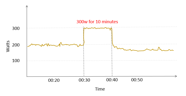
I rode at a moderate intensity of about 200w for 30 minutes then turned up the gas for 10 minutes at 300w. It turns out, according to the model above, that that 300w was a maximal effort. So we will try and find it.

Monotonicity

One of the really useful aspects of power (and heartrate) data is that it is impossible to record negative values. You are either generating power, or you are not. If we convert power to energy (joules, which is calculated as power x time) then we can accumulate that over the course of a ride.

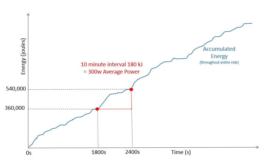
In the chart above you will see energy slowly increasing over time as the ride progresses. Indeed the interval we are looking for, starts at 1800s where 360kj of energy has been accumulated and ends at 2400s when a further 180kj of energy has been accumulated.

If we create an array of the accumulated energy throughout the ride we will be able to calculate the average power for any given interval with a single subtraction !

This insight was highlighted by Mark Rages in 2011 and forms the basis for a similar algorithm that finds best intervals for all durations in a ride.

Maximal efforts fall on the PD curve

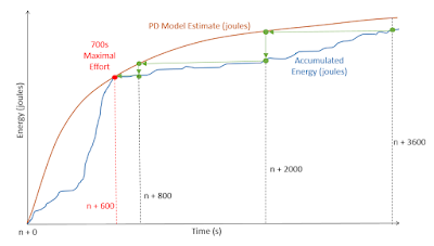
Looking at the chart below, you can see that if we compare the PD estimate in joules with the accumulated energy from any given point in a ride, the maximal effort will be where the two curves intersect (I have drawn the PD model estimate as a parabola as an aid to explain the algorithm, in reality it is linear and quite steep)

So we have now redefined the problem; we will look through a ride, from beginning to end, and at each point we will look for the interval that has an accumulated energy that is equal to (or higher) than the PD model estimated joules for that duration.

Scan back not forward

Clearly the trick above to compute the interval average with a single subtraction is going to be significantly faster than computing each one by iterating over the data. But it will still mean iterating for every interval length possible at every point in the ride.

So my insight into solving this problem was to start at the maximum interval length we are looking for and scan backwards. But crucially, we are going to exploit the monotonic nature of the data to skip those intervals that cannot possibly be maximal.

We are going to repeat the following process at every point within the ride. In the example above we are looking at point n=1800s which is, by no coincidence, the starting point for the maximal effort in our example.

First we compute the total joules for a 1hr (3600s) interval using the subtraction trick from above. Next, using our chosen power duration model we calculate the duration it would take to deplete the energy in a maximal effort.

In our case, over that 3600s we might have accumulated say, 360 kJ. The PD model tells us that a maximal effort of 2000 seconds would burn 360 kJ *. This is considerably shorter than the 3600s we are currently looking at. 

Now, because the accumulated series is monotonic we know that it is impossible for any values between 2000s and 3600s to be higher than the value at 3600s. So we can skip back to an interval of length 2000s and not bother checking intervals of length 2000-3600s from this point in the ride. 

As we repeat this scan back we jump back to 800s and more until eventually we find our maximal effort; the TTE returned by the PD model at 600s is equal to the 600s length of the interval we are at. So it is a maximal effort.

So, in our example above, we have found the maximal interval starting from 1800s into the ride in about 4 iterations. This will be repeated at every point in the ride, but typically we will only need to iterate a handful of times at each point in the ride.

In computational terms, we have moved from an algorithm of O(n²) time to one that iterates over all points but then only looks at a subset, more formally to a runtime of O(n log n).

In reality, this new approach performs dramatically faster for rides where the rider doesn't do any sustained efforts, because the scan back jumps back in a couple of iterations. When a ride contains lots of hard efforts then it can take longer. But in my experience so far the worst case is typcially 1:100 times faster than the brute force approach and the best case is 1:10000 times faster. It's a pretty neat trick.

* converting energy to a TTE duration means we take the power duration model formula and solve for time rather than for power. For example, the Monod and Scherrer formula is P(t) = W'/t + CP. If we convert that to joules we get Joules(t) = (W'/t + CP) * t. We can then take that and solve for t, in which case we end up with a rather elegant (and fast) t = (Joules - W') / CP.

But, the model is always wrong

Now, of course, in the real world the model is generally wrong. It is quite common to see efforts that exceed the estimates a fair amount. With training we get stronger and we don't always update our model parameters (CP, W' etc) to keep up.

So we end up with the situation below:

You can see that the model estimate is much lower than the actual performance. So we end up with a range of intervals from 400-600s long that are 'maximal'.

Now as it stands, our algorithm will stop when it finds the maximal effort at 600s, but if you look closely you will see that the accumulated energy from the "peak" doesn't rise. In other words, the 600s interval has a few zeroes at the end of it. From a user perspective this is quite odd.

So to address this, we cannot stop once we hit an interval that is TTE, we must keep going back, 1 second at a time, until we are no longer a TTE effort. As we do this we can calculate the 'quality' of the interval in relationship to the PD model and only keep  the interval at that "peak".

Once we get to 400s we will iterate back to 0 quite quickly and can stop searching.

Finally, Sustained intervals

So now we can apply exactly the same algorithm to find sustained intervals. Any 'near' maximal effort is clearly a sustained effort and we just need to define what we mean by 'near'. And for cases where the model is wrong, but predicting a slightly higher TTE than we are capable of it is very useful to seek values that are 'near' to the estimate.

By applying a bit of a tolerance we can account for when the model is over and under estimating the TTE we are capable of.

In the case of the implementation in GoldenCheetah, we have chosen to use 85% of maximal as a sustained effort and this seems to align to most user expectations so far.

We may tweak it later, but for now it seems to be working well and will be released alongside v3.2 in the next couple of months.

If you are interested in the code the algorithm can be found in RideItem::updateIntervals() in the source over at github.com.

Multiple Overlapping Efforts

The next problem to consider is, as shown in the case above, the situation where we have sustained efforts embedded within a longer one. It shows that whilst out doing a hearty 2hr tempo ride we perform a long vo2max interval of 6 minutes that also contains a near maximal sprint. Do select the best peak value (the vo2max effort in the middle) or are there actually 3 sustained efforts ?

That's for another blog post ...